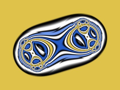
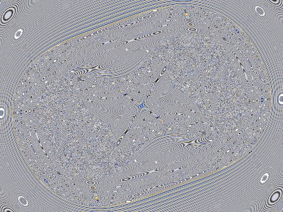
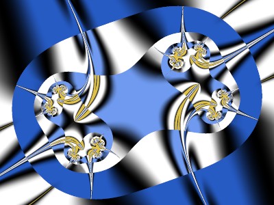
This is a follow-up to my previous Tutorial, “FormulaX Plug-ins”. If you haven’t read the introductory quote from the Ultra Fractal (UF) help file in that posting, do so now, and upload the latest version of the UF formulas. Here’s the upr and the image it produces.
1 {
::tBgk5in2Vi1WvNqOQ43rU/Pg49N12Byl9I/wmW1Va12VrUbli6LIXwk4zC2Iwstp/63JcJJA
mL9lEh/+mxzMemxDEmy81sove9VWWahOiTtx2WvJC07prwIr9cxu9aqrDyKidgnmRxW+p8Ah
Oja/DRs1moc+/Ruhs4GCi4YfUPMpWwiEsMhcH9AP76rKEtYP8ZJahSSt3w8/zuUVuMw2Slw8
F6DUMCd9VxskEQwS2cpmnSR3gsiZ7kU0s1g23BW5CgZoKNOPiVwMm9u4IVQFWhiIukFDuyja
mMglGMLPM22CUW6Bq935Seqw/+SpLs4EvKddbELDcs/P61Z5Rv+1f8zNeP+mQ7v3uFnZ/1bX
peKtaru4VPWYStBhA5xoAxBhxuGkePL7VmIi+LVHE1b07EgCgtXbQyQvNba6AbQI7eI20Laz
4ujmgKX3jHebNMaGChwth3An/+lH/dENJlTlKDr+8TjGYrZpTZysjIjwLPjnONu/RIDofLIw
Mq+QCn+ThkzS7VD5P1M0/8Te3nL9PmxbPgQT0nznubn/58cgeLLH56ryG0mfa4knSec8xi3e
VDnAJP4b6RYo0xosheV1uXWgD2d9DePA/zjeNVptHS8RD7Xy8iq5RYGUXdOVRy0sUdPxpzsS
8SUvBd4Ijyruu0ZIebbeef/2pG12O9w22pH32C29DFlYS1Y8y48AI14LoZujRtMkNSod749j
vg7p+aDtx9cKloy0ma8BLPlOf10Gtoum4k6AUSu3mflwj09rk0nt9XtUT1zz/EOf+n0//MtA
PLxUt8y+g9BW1FsfxL6E2B7ysbhMTEwLHjrwhBApSytyURiAqDZ1CX8csL56rgWDd5GVc0ei
9yVk5zX0zsU+RFRlmjT99UWgAW6WVkKFmfrKw5X9ohBrubIqducpNa9znj7dkvyiGl55ifCx
pDcZI50cMNBvsZQTkAVoQyi6TwwXe5c04lXsNRwUyVTSlzC3N8E+B9jP6y+89pto/8oFudEY
cjLsveVmo1TlaXqDUkag8IpRqwwM+FX92SDBCoddzcWvHvzuXuTImUR7O4Pm0nTJYMCveAqX
kciGgXAYYtMVE2eY+T1cz8ZQWmpk8S8Q4VIVpU3+1gQC+h+0V7tos534WvxyvP9KLdpOyR6r
YK2koJw6dWUirHSqdNfM/4RE9bRRdAfOj/gQ+A79e8nggYh0QRJsOITPR6j7oHLKiabB7Z32
BlzIa0Yh3IMmJPYMaE63KB+Wkr5IrvekAbZ7sfB3pYM8WOba3jj2vCZT4UuvIpciomAwP6ds
sk+3QvTUwmyTITPliMWKFpnUKiBHWSOeKVf3TxlsZxKlefRBEMcNr47fQIrsgJu4vTdmv2qQ
FUnlLW5s806LwVrXE5qWc18qFxLWucJB7WB4icNDghNqjawuoa2wgBrmvGVDsk0DwanuqhgX
aeTJn8p2AmcKyZnydJisAEuEYOaRPAmcq5ndqmb68zOVLg1udVzXqJ7sa9aXXAp6zTd5ZJkx
WyGd6jXRchGg/DgNNmoC
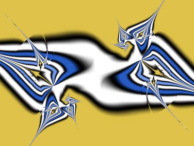
}
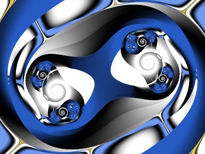
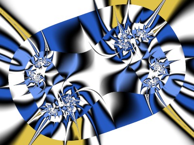
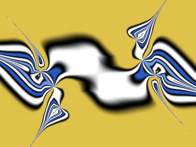
It’s the same fractal as in the third image of the previous tutorial, except on the Location tab, where the magnification is now 0.9 and the Rotation angle is now 60 degrees to make some of the following images fit better. I’ll keep the same Location settings, Gradient, and Formula settings for the rest of this tutorial, and only a single layer.
On the Outside tab, “Plug-In Coloring (Gradient)” comes from Standard.ucl and the plug-in “Color by Distance” comes from jlb.ulb.
For each pixel, UF calculates a series of z values using the Iteration part of a Formula. After each z is calculated (except just after the sequence has bailed out), UF calls the Coloring functions at the tops of the Inside and Outside tabs. (I’ll only deal with the Outside tab here.) The Iteration part of these Coloring functions may or may not do something with the z values.
After the series has bailed out, including the possibility of running out of the allowed number of iterations, UF calls the ResultIndex part of the plug-in; it calculates a number that is used as an index into the gradient for coloring. The end result of all this is, for each pixel, to convert a series of complex numbers into one number, the index. I’ve defined a new Distance class whose Iteration step converts a complex number into a real number, a float.
Thus the title of the “Coloring Algorithm”, “Color by Distance”. Some of the Distances are actual distances. For example, “D01 cabs” is the diagonal distance from z to the origin. If z is (x,y), then D01 gives sqrt(x^2 + y^2). “D04 |Real|+|Imag|” is the distance from z to the origin going only horizontally and vertically; D04 gives abs(x)+abs(y). (It’s like “manh”, short for Manhattan, referring to New York City blocks, which is often found in ufm formulas as part of bailout settings.) Other Distances may also be real distances, such as from z to a circle or rectangle. Other Distances may have no relation to real distances, but are just ways to convert a complex number to a float.
The Basic version of Color by Distance has two phases. In the Accumulation phase, after each z is calculated by the formula, the Distance plugin does something useful, accumulating information about the z sequence. In the Final phase, this accumulated information is used to provide an index into the gradient for coloring the pixel. For example, “C05 Distance range” sets the index to the largest distance minus the smallest distance.
Below the line “D01 cabs” is “Scale?”. Click on this.
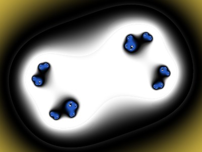
What happened? Since the Julia-type Mandelbrot formula is divergent, the z values get larger and larger as the sequence progresses. The distances get larger and larger.
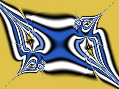
The scaling for D01 uses the tanh function to keep the index within range. The “Scale factor” is the value that gives an index value of tanh(1), approximately 0.76. Experiment.
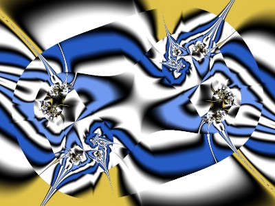
Another way to deal with Too Much Detail (TMD) is to use “Final smooth”. Keep Scale unchecked and choose “Mandelbrot type” with parameters 2 and 100, matching the Formula tab.
This is the smoothing used by "Smooth (Mandelbrot)" coloring in Standard.ucl and in Standard.ufm. Changing parameters can be useful. Experiment. The other smoothing, “TIA type”, is that used by "Triangle Inequality Average" coloring, also in Standard.ucl and in Standard.ufm. It sometimes gives interesting results. Experiment.
Go back to Final smooth of “None”. Another way to deal with TMD is to change the “Color Density” or “Transfer Function”. Leave the Color Density at 1 and change the Transfer Function to “CubeRoot”.
Go back to the original settings.
The “Simple distance” plug-in has 21 plug-ins that can convert z to a number. Click on the Browser button to the right of “Use for distance” to see their thumbnails. When used in Color by Distance, only the absolute values are used. For example, “D08 Real-Imag”, for z = (x,y), means abs(x-y). Most of these should be self-explanatory, except for the last two.
For D02 through D18 you have the option of scaling the distances. For “D02 Real” this means coloring according to abs(x)/sqrt(x^2+y*2) instead of by abs(x). This gives different results from smoothing and from changing the Color Density or Transfer Function. Experiment.
For “D19 Path ratio”, think of the sequence of z values as being connected by straight lines in the xy plane, from the first z value to the current z value. The path ratio is the sum of these straight line distances, divided by the straight line distance from the first z value to the current z value. It’s never larger than one. Because it is exactly one at the first iteration, the colorings “C01 First distance” and “C04 Largest distance” always give a uniform color—not interesting.
For “D20 Angle”, the usual angle calculated using the UF function atan2 is divided by 2*pi and shifted to keep the value in the range 0 to 1. There are two different versions. Type 1 is the usual one.
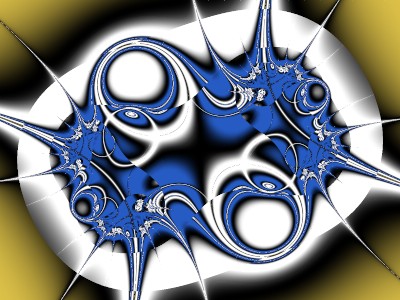
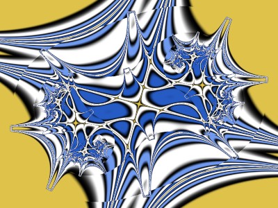
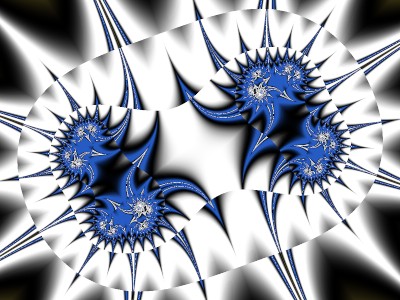
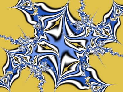
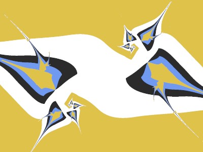
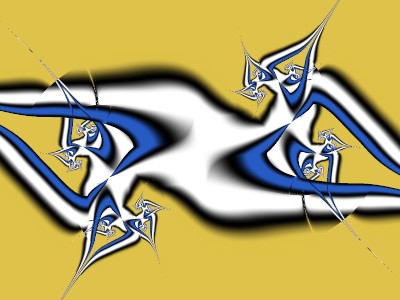
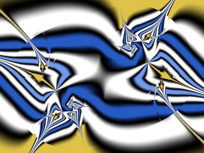
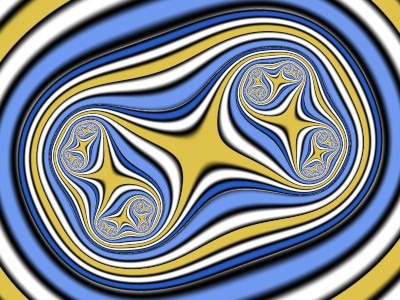
Experiment. For example, here is the result if “Use for distance” is “D11 Real/Imag”, “Scale” is checked, coloring is “C05 Distance Range”, and no Final smooth,
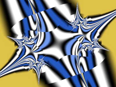
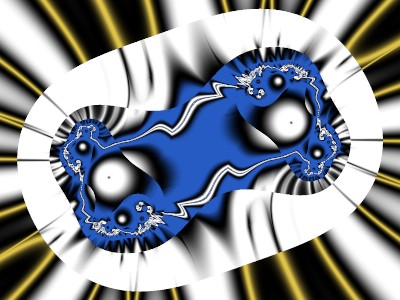
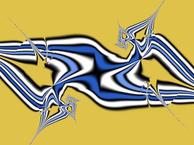
And with Mandelbrot-type Final smooth and Color Density of 2 instead of 1.
Experiment. Then go back to the original parameters, with “D01 cabs”, Scale checked, and “C05 Distance range”.
In the “How to color” part of Color by Distance there are 13 ways of coloring. Click on the Browser button on the “How to color” line to see the thumbnails. The first four are self-explanatory and the fifth was already explained. “C06 Distance ratio” calculates the largest distance divided by the smallest distance. For this fractal, C06 gives TMD and can use a Mandelbrot-type final smooth. Experiment. “C07 Iteration count” calculates the number of iterations divided by the scale. Not too interesting for this fractal.
The next three coloring methods are averages. Roughly speaking, “C08 Arithmetic average” emphasizes the larger distances, “C10 Harmonic average” emphasizes the smaller distances,, and “C09 Geometric average” is in between. Experiment.
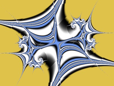
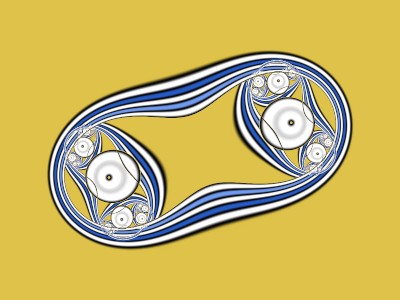
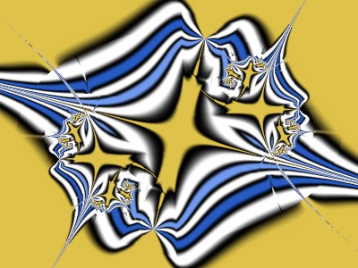
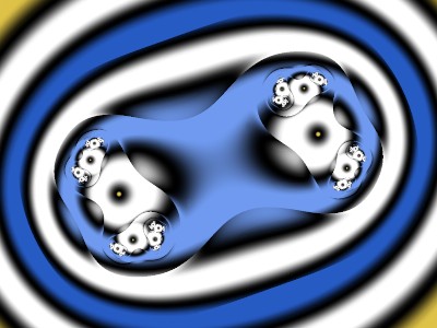
The next three coloring methods are variations on C08. (For the mathematicians among us, C11 is the standard deviation, C12 is the coefficient of variation, and C13 is approximately the fractal dimension.) Experiment. Often C13 can benefit from a Color Density that’s larger or a Transfer Function of Sqr or Cube. Here’s C!3 with Color Density 2 and Transfer Function Sqr.
[continued in next message]
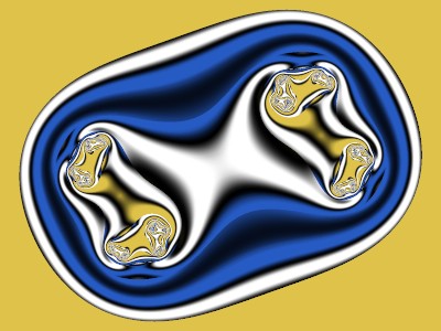
This is a follow-up to my previous Tutorial, “FormulaX Plug-ins”. If you haven’t read the introductory quote from the Ultra Fractal (UF) help file in that posting, do so now, and upload the latest version of the UF formulas. Here’s the upr and the image it produces.
1 {
::tBgk5in2Vi1WvNqOQ43rU/Pg49N12Byl9I/wmW1Va12VrUbli6LIXwk4zC2Iwstp/63JcJJA
mL9lEh/+mxzMemxDEmy81sove9VWWahOiTtx2WvJC07prwIr9cxu9aqrDyKidgnmRxW+p8Ah
Oja/DRs1moc+/Ruhs4GCi4YfUPMpWwiEsMhcH9AP76rKEtYP8ZJahSSt3w8/zuUVuMw2Slw8
F6DUMCd9VxskEQwS2cpmnSR3gsiZ7kU0s1g23BW5CgZoKNOPiVwMm9u4IVQFWhiIukFDuyja
mMglGMLPM22CUW6Bq935Seqw/+SpLs4EvKddbELDcs/P61Z5Rv+1f8zNeP+mQ7v3uFnZ/1bX
peKtaru4VPWYStBhA5xoAxBhxuGkePL7VmIi+LVHE1b07EgCgtXbQyQvNba6AbQI7eI20Laz
4ujmgKX3jHebNMaGChwth3An/+lH/dENJlTlKDr+8TjGYrZpTZysjIjwLPjnONu/RIDofLIw
Mq+QCn+ThkzS7VD5P1M0/8Te3nL9PmxbPgQT0nznubn/58cgeLLH56ryG0mfa4knSec8xi3e
VDnAJP4b6RYo0xosheV1uXWgD2d9DePA/zjeNVptHS8RD7Xy8iq5RYGUXdOVRy0sUdPxpzsS
8SUvBd4Ijyruu0ZIebbeef/2pG12O9w22pH32C29DFlYS1Y8y48AI14LoZujRtMkNSod749j
vg7p+aDtx9cKloy0ma8BLPlOf10Gtoum4k6AUSu3mflwj09rk0nt9XtUT1zz/EOf+n0//MtA
PLxUt8y+g9BW1FsfxL6E2B7ysbhMTEwLHjrwhBApSytyURiAqDZ1CX8csL56rgWDd5GVc0ei
9yVk5zX0zsU+RFRlmjT99UWgAW6WVkKFmfrKw5X9ohBrubIqducpNa9znj7dkvyiGl55ifCx
pDcZI50cMNBvsZQTkAVoQyi6TwwXe5c04lXsNRwUyVTSlzC3N8E+B9jP6y+89pto/8oFudEY
cjLsveVmo1TlaXqDUkag8IpRqwwM+FX92SDBCoddzcWvHvzuXuTImUR7O4Pm0nTJYMCveAqX
kciGgXAYYtMVE2eY+T1cz8ZQWmpk8S8Q4VIVpU3+1gQC+h+0V7tos534WvxyvP9KLdpOyR6r
YK2koJw6dWUirHSqdNfM/4RE9bRRdAfOj/gQ+A79e8nggYh0QRJsOITPR6j7oHLKiabB7Z32
BlzIa0Yh3IMmJPYMaE63KB+Wkr5IrvekAbZ7sfB3pYM8WOba3jj2vCZT4UuvIpciomAwP6ds
sk+3QvTUwmyTITPliMWKFpnUKiBHWSOeKVf3TxlsZxKlefRBEMcNr47fQIrsgJu4vTdmv2qQ
FUnlLW5s806LwVrXE5qWc18qFxLWucJB7WB4icNDghNqjawuoa2wgBrmvGVDsk0DwanuqhgX
aeTJn8p2AmcKyZnydJisAEuEYOaRPAmcq5ndqmb68zOVLg1udVzXqJ7sa9aXXAp6zTd5ZJkx
WyGd6jXRchGg/DgNNmoC
}

It’s the same fractal as in the third image of the previous tutorial, except on the Location tab, where the magnification is now 0.9 and the Rotation angle is now 60 degrees to make some of the following images fit better. I’ll keep the same Location settings, Gradient, and Formula settings for the rest of this tutorial, and only a single layer.
On the Outside tab, “Plug-In Coloring (Gradient)” comes from Standard.ucl and the plug-in “Color by Distance” comes from jlb.ulb.
For each pixel, UF calculates a series of z values using the Iteration part of a Formula. After each z is calculated (except just after the sequence has bailed out), UF calls the Coloring functions at the tops of the Inside and Outside tabs. (I’ll only deal with the Outside tab here.) The Iteration part of these Coloring functions may or may not do something with the z values.
After the series has bailed out, including the possibility of running out of the allowed number of iterations, UF calls the ResultIndex part of the plug-in; it calculates a number that is used as an index into the gradient for coloring. The end result of all this is, for each pixel, to convert a series of complex numbers into one number, the index. I’ve defined a new Distance class whose Iteration step converts a complex number into a real number, a float.
Thus the title of the “Coloring Algorithm”, “Color by Distance”. Some of the Distances are actual distances. For example, “D01 cabs” is the diagonal distance from z to the origin. If z is (x,y), then D01 gives sqrt(x^2 + y^2). “D04 |Real|+|Imag|” is the distance from z to the origin going only horizontally and vertically; D04 gives abs(x)+abs(y). (It’s like “manh”, short for Manhattan, referring to New York City blocks, which is often found in ufm formulas as part of bailout settings.) Other Distances may also be real distances, such as from z to a circle or rectangle. Other Distances may have no relation to real distances, but are just ways to convert a complex number to a float.
The Basic version of Color by Distance has two phases. In the Accumulation phase, after each z is calculated by the formula, the Distance plugin does something useful, accumulating information about the z sequence. In the Final phase, this accumulated information is used to provide an index into the gradient for coloring the pixel. For example, “C05 Distance range” sets the index to the largest distance minus the smallest distance.
Below the line “D01 cabs” is “Scale?”. Click on this.

What happened? Since the Julia-type Mandelbrot formula is divergent, the z values get larger and larger as the sequence progresses. The distances get larger and larger.
The scaling for D01 uses the tanh function to keep the index within range. The “Scale factor” is the value that gives an index value of tanh(1), approximately 0.76. Experiment.
Another way to deal with Too Much Detail (TMD) is to use “Final smooth”. Keep Scale unchecked and choose “Mandelbrot type” with parameters 2 and 100, matching the Formula tab.

This is the smoothing used by "Smooth (Mandelbrot)" coloring in Standard.ucl and in Standard.ufm. Changing parameters can be useful. Experiment. The other smoothing, “TIA type”, is that used by "Triangle Inequality Average" coloring, also in Standard.ucl and in Standard.ufm. It sometimes gives interesting results. Experiment.
Go back to Final smooth of “None”. Another way to deal with TMD is to change the “Color Density” or “Transfer Function”. Leave the Color Density at 1 and change the Transfer Function to “CubeRoot”.

Go back to the original settings.
The “Simple distance” plug-in has 21 plug-ins that can convert z to a number. Click on the Browser button to the right of “Use for distance” to see their thumbnails. When used in Color by Distance, only the absolute values are used. For example, “D08 Real-Imag”, for z = (x,y), means abs(x-y). Most of these should be self-explanatory, except for the last two.
For D02 through D18 you have the option of scaling the distances. For “D02 Real” this means coloring according to abs(x)/sqrt(x^2+y*2) instead of by abs(x). This gives different results from smoothing and from changing the Color Density or Transfer Function. Experiment.
For “D19 Path ratio”, think of the sequence of z values as being connected by straight lines in the xy plane, from the first z value to the current z value. The path ratio is the sum of these straight line distances, divided by the straight line distance from the first z value to the current z value. It’s never larger than one. Because it is exactly one at the first iteration, the colorings “C01 First distance” and “C04 Largest distance” always give a uniform color—not interesting.
For “D20 Angle”, the usual angle calculated using the UF function atan2 is divided by 2*pi and shifted to keep the value in the range 0 to 1. There are two different versions. Type 1 is the usual one.
Experiment. For example, here is the result if “Use for distance” is “D11 Real/Imag”, “Scale” is checked, coloring is “C05 Distance Range”, and no Final smooth,

And with Mandelbrot-type Final smooth and Color Density of 2 instead of 1.

Experiment. Then go back to the original parameters, with “D01 cabs”, Scale checked, and “C05 Distance range”.
In the “How to color” part of Color by Distance there are 13 ways of coloring. Click on the Browser button on the “How to color” line to see the thumbnails. The first four are self-explanatory and the fifth was already explained. “C06 Distance ratio” calculates the largest distance divided by the smallest distance. For this fractal, C06 gives TMD and can use a Mandelbrot-type final smooth. Experiment. “C07 Iteration count” calculates the number of iterations divided by the scale. Not too interesting for this fractal.
The next three coloring methods are averages. Roughly speaking, “C08 Arithmetic average” emphasizes the larger distances, “C10 Harmonic average” emphasizes the smaller distances,, and “C09 Geometric average” is in between. Experiment.
The next three coloring methods are variations on C08. (For the mathematicians among us, C11 is the standard deviation, C12 is the coefficient of variation, and C13 is approximately the fractal dimension.) Experiment. Often C13 can benefit from a Color Density that’s larger or a Transfer Function of Sqr or Cube. Here’s C!3 with Color Density 2 and Transfer Function Sqr.

[continued in next message]