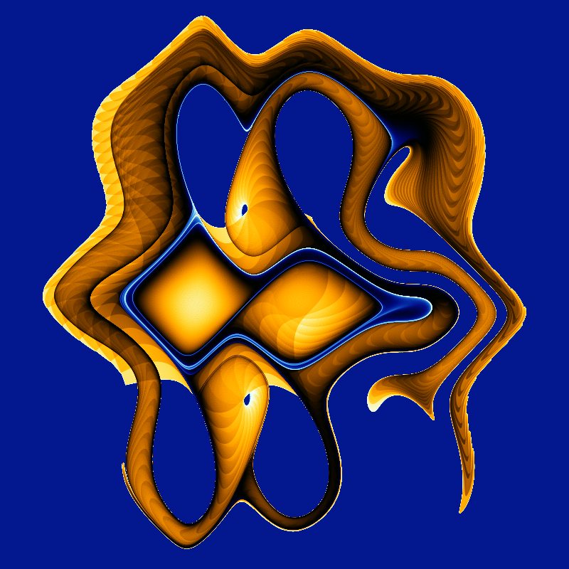
Find it in mt5.ucl.
This coloring algorithm is based on Chapter 14 of Clifford Pickover's book Computers, Chaos, Pattern and Beauty, where here introduced "Popcorn" and a number related gnarly equations. The rendering method used in the book, and here, is similar to that used by Flame Fractals. This doesn't suit Ultra Fractal's native method of calculating fractals, so the whole process has to be done in a coloring algorithm.
Since I'm math-challenged I won't try to explain the equations that Pickover uses. The first one he describes goes in UF style pseudocode:
Xnew = x - h * sin(y + sin(p * y))
Ynew = y + h * sin(x + sin(p * x))
Notice that the same function is used on both sides of the equation.
Many people have played with changing these equations, looking for something new and interesting. I've had a lot of succsess using variatios of them. But rather that writing lots of different equations into the coloring algorithm I decided to implement them as plug-ins. I've also made it so that you can load different functions into both sides of the equation.
I've also included the ability to supply the plug-in functions with "noise" wich they can use in whatever manner they wish, and a transform to distort the equations. Both of these need to be calculation for every iteration, so they can slow things down.
The algorithm works by choosing (sampling) a large number of points within a defined area of the x-y plane (the sample area). The sampled points are iterated through the equations a number of times, and the resulting orbits are plotted to the (virtual) screen. A count is kept of how many times each pixel is "hit" by an orbit and the results are finally scaled to a value between 0 and 1 to index the gradient.
To get started use "Pixel" in mt.ufm for the fractal formula and "Dynamical Systems" in mt5.ucl for the outside coloring algorithm. Open the gradient tool and replace the gradient with "Lighting" from Standard.ugr and then select the menu item Gradient > Reverse. You can then add and adjust control points to get the balance that you like. Set the Drawing Method to one of the linear modes.
High resolution images can take a long time to render.
The parameters:
Sample Mode determines the way the sample points are chosen. In the "Grid" mode the points are spread evenly over the sample area in a grid. In the "Random" mode the points are chosen at random. The same number of points are sampled in both modes so there's little difference in quality, but some details may differ.
Center is the center of the sample area. Change this to concentrate on a certain area of the x-y plane. Since orbits can be unpredictable you may need to experiment a but.
Width is the width of the sample area. The sample area is a square unless Circular Mask is enabled. If you zoom into the image try adjusting the width so that the sample area is just big enough to cover the area you're interested in.
Step Size is used in the equation ("h" in the example above) and as the name suggests it affects the distance between points in an orbit. As you increase this parameter the image can become more chaotic and a higher Resolution may be needed.
Iterations is the number of times a sample point is iterated, and so the length of the orbit. Depending on the functions used, orbits will wander outside the sample area. You can often see these branches grow by increasing the iterations. Higher Iterations can bring out or cover up detail, and won't necessarily increase the density of points in the image area. Iterations can have a large effect rendering time, especially when Resolution is high.
Resolution determines how many points are sampled. The higher the resolution the more points are sampled, and the image becomes less grainy. It's important to remember that the resolution applies to the sample area, not the image area, so that if you decrease the size of the sample area all of the points will be compressed into that smaller area. Resolution gives a fixed number of sample points so if you increase the size of the image you'll need to increase Resolution as well. Resolution has a large effect on the time it takes to render an image.
Circular Mask. With this parameter enabled the sample area is masked with a circle. Points outside the circle aren't sampled. However orbits that travel outside the circle are still plotted. Use this when the square shape of the sample area is too obvious for your purposes.
Dual Functions. If this is enabled you can load a different function on the two sides of the equation. Otherwise the plug-in loaded into X Function is used on both sides
X Function. This is where you load the function plug-in for the X side of the equation. Click the Browse button and navigate to mt.ulb to find some supplied functions. Since the Dynamical Function class was created for this purpose anything visible in the browser is suitable. If the plug-in has it's own parameters they will appear below the function name.
Y Function. This is where you load the function plug-in for the Y side of the equation and will only be visible if Dual Functions is enabled. Don't worry about whether functions belong together: the idea was to mix and match things to see what happens.
Add Noise. If this is enabled some "noise" is generated and sent to the functions. A slot will appear where you can load an MT_TextureColoring plug-in. The plug-in will have it's own set of parameters. It's up to the function plug-in to use the noise and it will have no effect on most functions. Noise is calculated every iteration so it will increase render time.
Noise Amount is only visible when Add Noise is enabled. This is the amount or strength of the noise. Higher values will have a more obvious effect.
Noise Scale is only visible when Add Noise is enabled. The MT_TextureColoring class returns a floating point value based on a point in the x-y plane. Increasing this value "zooms out" on the texture, and decreasing it "zooms in". Since the function plug-in can do what it wants with this noise value you'll need to experiment.
Add Transform. If this parameter is enabled a transform is added to the calculation after the function plug-in. A slot appears where you can load a UserTransform plug-in. If the plug-in has parameters they will appear below. Since the transform is added to the calculation on every iteration the effect may not be as the transform author intended. Adding a transform can increase render time considerably.
Find it in mt5.ucl.
This coloring algorithm is based on Chapter 14 of Clifford Pickover's book _Computers, Chaos, Pattern and Beauty_, where here introduced "Popcorn" and a number related gnarly equations. The rendering method used in the book, and here, is similar to that used by Flame Fractals. This doesn't suit Ultra Fractal's native method of calculating fractals, so the whole process has to be done in a coloring algorithm.
Since I'm math-challenged I won't try to explain the equations that Pickover uses. The first one he describes goes in UF style pseudocode:
````
Xnew = x - h * sin(y + sin(p * y))
Ynew = y + h * sin(x + sin(p * x))
````
Notice that the same function is used on both sides of the equation.
Many people have played with changing these equations, looking for something new and interesting. I've had a lot of succsess using variatios of them. But rather that writing lots of different equations into the coloring algorithm I decided to implement them as plug-ins. I've also made it so that you can load different functions into both sides of the equation.
I've also included the ability to supply the plug-in functions with "noise" wich they can use in whatever manner they wish, and a transform to distort the equations. Both of these need to be calculation for every iteration, so they can slow things down.
The algorithm works by choosing (sampling) a large number of points within a defined area of the x-y plane (the sample area). The sampled points are iterated through the equations a number of times, and the resulting orbits are plotted to the (virtual) screen. A count is kept of how many times each pixel is "hit" by an orbit and the results are finally scaled to a value between 0 and 1 to index the gradient.
To get started use "Pixel" in mt.ufm for the fractal formula and "Dynamical Systems" in mt5.ucl for the outside coloring algorithm. Open the gradient tool and replace the gradient with "Lighting" from Standard.ugr and then select the menu item Gradient > Reverse. You can then add and adjust control points to get the balance that you like. Set the Drawing Method to one of the linear modes.
High resolution images can take a long time to render.
The parameters:
**Sample Mode** determines the way the sample points are chosen. In the "Grid" mode the points are spread evenly over the sample area in a grid. In the "Random" mode the points are chosen at random. The same number of points are sampled in both modes so there's little difference in quality, but some details may differ.
**Center** is the center of the sample area. Change this to concentrate on a certain area of the x-y plane. Since orbits can be unpredictable you may need to experiment a but.
**Width** is the width of the sample area. The sample area is a square unless Circular Mask is enabled. If you zoom into the image try adjusting the width so that the sample area is just big enough to cover the area you're interested in.
**Step Size** is used in the equation ("h" in the example above) and as the name suggests it affects the distance between points in an orbit. As you increase this parameter the image can become more chaotic and a higher Resolution may be needed.
**Iterations** is the number of times a sample point is iterated, and so the length of the orbit. Depending on the functions used, orbits will wander outside the sample area. You can often see these branches grow by increasing the iterations. Higher Iterations can bring out or cover up detail, and won't necessarily increase the density of points in the image area. Iterations can have a large effect rendering time, especially when Resolution is high.
**Resolution** determines how many points are sampled. The higher the resolution the more points are sampled, and the image becomes less grainy. It's important to remember that the resolution applies to the sample area, not the image area, so that if you decrease the size of the sample area all of the points will be compressed into that smaller area. Resolution gives a fixed number of sample points so if you increase the size of the image you'll need to increase Resolution as well. Resolution has a large effect on the time it takes to render an image.
**Circular Mask.** With this parameter enabled the sample area is masked with a circle. Points outside the circle aren't sampled. However orbits that travel outside the circle are still plotted. Use this when the square shape of the sample area is too obvious for your purposes.
**Dual Functions.** If this is enabled you can load a different function on the two sides of the equation. Otherwise the plug-in loaded into X Function is used on both sides
**X Function**. This is where you load the function plug-in for the X side of the equation. Click the Browse button and navigate to mt.ulb to find some supplied functions. Since the Dynamical Function class was created for this purpose anything visible in the browser is suitable. If the plug-in has it's own parameters they will appear below the function name.
**Y Function.** This is where you load the function plug-in for the Y side of the equation and will only be visible if Dual Functions is enabled. Don't worry about whether functions belong together: the idea was to mix and match things to see what happens.
**Add Noise.** If this is enabled some "noise" is generated and sent to the functions. A slot will appear where you can load an MT_TextureColoring plug-in. The plug-in will have it's own set of parameters. It's up to the function plug-in to use the noise and it will have no effect on most functions. Noise is calculated every iteration so it will increase render time.
**Noise Amount** is only visible when Add Noise is enabled. This is the amount or strength of the noise. Higher values will have a more obvious effect.
**Noise Scale** is only visible when Add Noise is enabled. The MT_TextureColoring class returns a floating point value based on a point in the x-y plane. Increasing this value "zooms out" on the texture, and decreasing it "zooms in". Since the function plug-in can do what it wants with this noise value you'll need to experiment.
**Add Transform.** If this parameter is enabled a transform is added to the calculation after the function plug-in. A slot appears where you can load a UserTransform plug-in. If the plug-in has parameters they will appear below. Since the transform is added to the calculation on every iteration the effect may not be as the transform author intended. Adding a transform can increase render time considerably.